Remember that Analysis of Variance (ANOVA) is using linear regression to analyze how discrete input variables affect an outcome. Because the input variables are comprised of discrete “levels” (e.g., treatment groups), we are really comparing how the mean of an outcome varies among discrete groups. This is therefore a generalization of two-sample \(t\)-tests to the case of more than two samples/groups.
One-way ANOVA is the special case in which we only have one input variable, which has more than two “levels”. The ANOVA linear model can be written in several ways, but for me the easiest way to think about is as follows: \[y_{i,l} = \mu_l + \epsilon_{i,l}\]\[\epsilon \sim N(0, \sigma^2 I)\]
In this case \(l = 1,\dots,L\), where \(L\) is the number of levels in the input variable \(x\), and \(\mu_l\) is the mean outcome of group level, \(l\). Thus, each data observation \(y_{i,l}\) varies about a group level mean, with residuals \(\epsilon_{i,l}\), which are normally and independently distributed.
Perhaps this is easier to visualize and see the code. Let’s simulate a case in which we have a single input variable \(x\) that has 3 levels.
set.seed(5)n_levels=3n_obs_per_level=25# Construct Xx=rep(c(1:n_levels), each =n_obs_per_level)# Assign group-wise meansmus=NULLmus[1]=5.0mus[2]=7.5mus[3]=5.8sigma=2.5# residual sigma# Simulate data obsy=NULLfor(iin1:length(x)){this_level=x[i]y[i]=mus[this_level]+# residual deviation from group-wise mean:rnorm(1, mean =0, sd =sigma)}# Store in data frameone_way_df=data.frame( y =y, x =factor(x)# store as factor/categorical)# Plot the means:## Defaults to boxplot() when x is discreteplot(y~x, data =one_way_df)
We can see that - at least visually - level 2 has a higher mean outcome than the other levels (e.g., \(\bar{y}_2\) seems largest). Let’s run the ANOVA model and see the summary.
# Use the aov() functionm_one_way=aov(y~1+x, data =one_way_df)summary(m_one_way)
            Df Sum Sq Mean Sq F value   Pr(>F)
x            2  125.5   62.74   10.32 0.000115 ***
Residuals   72  437.9    6.08
---
Signif. codes:  0 '***' 0.001 '**' 0.01 '*' 0.05 '.' 0.1 ' ' 1
8.1.1 Manually calculate \(F\)
As we can see, the aov() function is using an \(F\)-test to determine if any of the group-wise means differ from the global mean (see lecture materials on this topic). Indeed, based on the \(p\)-value, at least one group-wise mean is different. To verify our understand, as usual, let’s manually calculate the \(F\) test statistic and \(p\)-value.
# First, we need to run the "null" model (intercept only)m_one_way_null=lm(y~1, data =one_way_df)# Extract the residuals (errors)resid_full=m_one_way$residualsresid_null=m_one_way_null$residuals# Sum of Square Errors (SSE)sse_full=crossprod(resid_full)sse_null=crossprod(resid_null)# degrees of freedomn_obs=length(y)df_full=n_obs-n_levelsdf_null=n_obs-1# Calculate F_statf_test=((sse_null-sse_full)/(df_null-df_full))/(sse_full/df_full)# Degrees of freedom for the F distribution:df_numerator=df_null-df_fulldf_denominator=df_fullp_one_way=1-pf(f_test, df1 =df_numerator, df2 =df_denominator)# Compare to anova()f_test; p_one_way
We see that our manual calculation of \(F\) and the corresponding \(p\)-value match with the output of the aov() function, so we can verify we are understanding what aov() is doing.
8.1.2 Tukey HSD
But, which specific means differ from each other? To know this, we need to compute all pairwise differences between the group-wise means. Remember that for \(L\) number of groups, we have \(L(L-1)/2\) number of pairwise comparisons. We want to correct for multiple comparisons, so we don’t inflate our risk of Type I errors. Therefore, we’ll conduct a Tukey Honest Significant Difference (HSD) test.
  Tukey multiple comparisons of means
    95% family-wise confidence level

Fit: aov(formula = y ~ 1 + x, data = one_way_df)

$x
          diff       lwr        upr     p adj
2-1  2.9796804  1.310442  4.6489184 0.0001710
3-1  0.5570861 -1.112152  2.2263241 0.7050400
3-2 -2.4225942 -4.091832 -0.7533562 0.0024902
This test is looking at pairwise differences. For instance 2-1 is the difference between \(x\) levels 2 and 1, and so on. The output reports the raw difference in means as diff, and then reports the lower and upper confidence limits of this difference as lwr and upr. These default to 95% confidence intervals, though the user can specify an option in the function to change this percentage confidence. Then the output reports the p adj, which is the adjusted \(p\)-value, adjusting for multiple comparisons. Here, we can conclude that while levels 1 and 3 are not different from one another, level 2 is different from both levels 1 and 3. This makes sense when we look at the boxplot (again).
How does the Tukey HSD adjust for multiple comparisons? It uses a special hypothesis test, which has an associated probability distribution, tukey. Remember that we calculate a test statistic, \(q\) for the difference between levels \(i\) and \(j\): \[q_{i,j} = \frac{|\bar{y}_i - \bar{y}_j|}{\sqrt{\hat{\sigma}^2_p/n}}\] Here, \(\hat{\sigma}^2_p\) is the pooled variance of the whole outcome data set, \(y\), and \(n\) is the number of observations per level. This is why a balanced design is important; the test assumes that each level has the same number of observations.
Let’s manually calculate the \(p\)-value for the difference between group levels 2 and 1.
# Need to extract the data observations associated with all x levels, separatelythese_x_1=which(x==1)these_x_2=which(x==2)these_x_3=which(x==3)y_1=y[these_x_1]y_2=y[these_x_2]y_3=y[these_x_3]# Calculate pooled variance for whole data set# Notice how this is not the same as var(y)pooled_var=(var(y_1)+var(y_2)+var(y_3))/3# Calculate q test statisticq_test=abs(mean(y_1)-mean(y_2))/sqrt(pooled_var/n_obs_per_level)q_test
[1] 6.041317
# Degrees of freedom for q test statdf_q=n_obs-n_levels# Calculate p-valuep_2v1=ptukey(q_test, nmeans =3, df =df_q, lower.tail =FALSE)p_2v1
[1] 0.0001710377
We can see this \(p\)-value matches the first p adj from the TukeyHSD() output.
8.2 Two-way ANOVA
Two-way ANOVA is the special case in which we have exactly two input variables, each of which has two or more “levels”. The two-way ANOVA linear model can be written in several ways. We’ll start with the easiest case in which each of the two input variables only has two levels. This refers to a “2x2” experimental design. To be concrete, we’ll use an example. We will simulate data for plant growth in which we manipulate Temperature (Low or High) and soil Moisture (Dry or Wet). We apply the 2x2 combination of these treatments which leads to four total treatments (e.g., Low-Dry, Low-Wet, etc.). We will apply each treatment combination to 25 plants and measure the outcome of Growth.
In the following model structure, we will code Temperature as Low == 0 and High == 1, and we will code soil Moisture as Dry == 0 and Wet == 1.
In the model structure, \(\mu\) is a global mean for \(y\) (i.e., across all treatments). Then, this global mean can be altered (i.e. affected by) the treatment combinations. \(\beta_{\text{Temp}}\) and \(\beta_{\text{Moist}}\) are the “main” effects and \(\beta_{\text{Intx}}\) is the interactive effect. Temp and Moist are binary indicator variables (0/1), so, for instance, if Temperature is Low, Temp == 0, and so on. This means that \(\beta_{\text{Temp}}\) only gets added to the global mean when Temp == 1 (i.e., Temperature is High), and so on. The \(\beta_{\text{Intx}}\) would get added to the global mean if both Temp and Moist are 1, so High Temperature and Wet Moisture.
8.2.1 Only main effects
First, let’s simulate a case in which we only have main effects, no interaction. Specifically, we will assume that the plant Growth declines under High Temperature, but that there is no effect of soil Moisture. Also, for data visualization, we will use the ggplot2 package, because it is easier to customize.
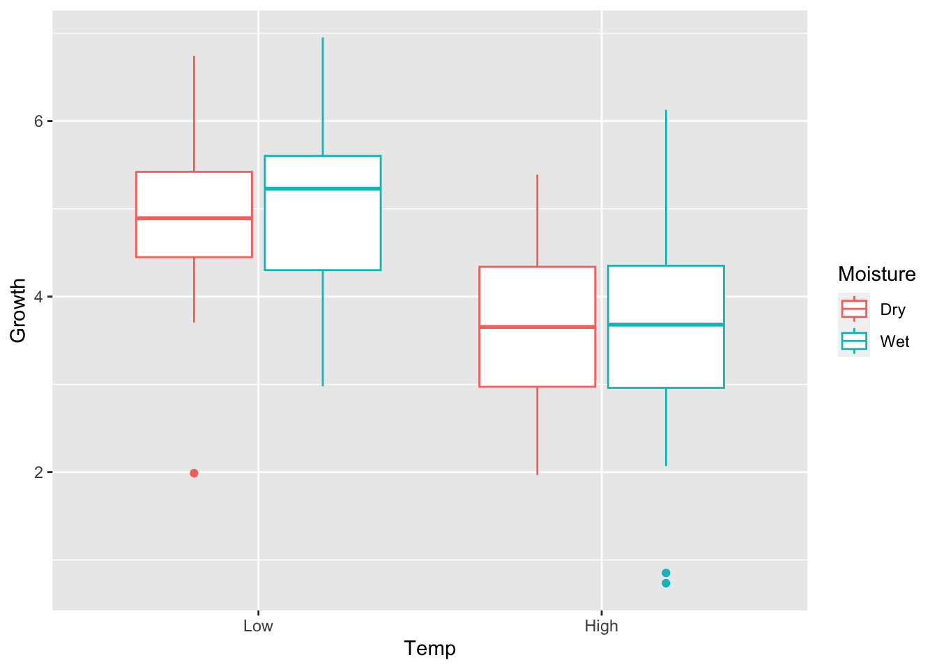
library(ggplot2)# 2x2 design# Replicated 25 times# Low, High (0, 1)n_reps=25Temp=rep(0:1, each =n_reps*2)# Low, High (0, 1)Moisture=c(rep(0:1, each =n_reps),rep(0:1, each =n_reps))# Simulate different effects:set.seed(8)# Just main effectglobal=5beta_t=-1.25beta_m=0beta_intx=0sigma=1.0y=NULLfor(iin1:length(Temp)){y[i]=global+beta_t*Temp[i]+beta_m*Moisture[i]+beta_intx*Temp[i]*Moisture[i]+rnorm(1, mean =0, sd =sigma)}# Store as data frametwo_way_df1=data.frame( Growth =y, Temp =factor(Temp, levels =c(0,1), labels =c("Low", "High")), Moisture =factor(Moisture, levels =c(0,1), labels =c("Dry", "Wet")))ggplot(two_way_df1)+geom_boxplot(aes(x =Temp, y =Growth, color =Moisture))
Here, it is visually clear that higher temperatures lead to lower plant growth, but there is no clear effect of soil moisture, just as we simulated.
Let’s run the ANOVA model and see if the output makes sense.
summary(aov(Growth~Temp+Moisture+Temp:Moisture, data =two_way_df1))
Indeed, we only see a main effect of Temp, and no main effect of Moisture, and no interactive effect (Temp:Moisture).
8.2.2 Interactive effect
Now will simulate a case in which we have a main effect of temperature, similar to the above (Growth declines at High Temp). We will also add a positive interactive effect. This means that the effect of specific effects of temperature on growth will depend on the soil moisture content. Specifically, with a positive interactive effect, if Temperature is High and Moisture is Wet, then we will get an increase in Growth, rather than a decline. Let’s see what this looks like visually.
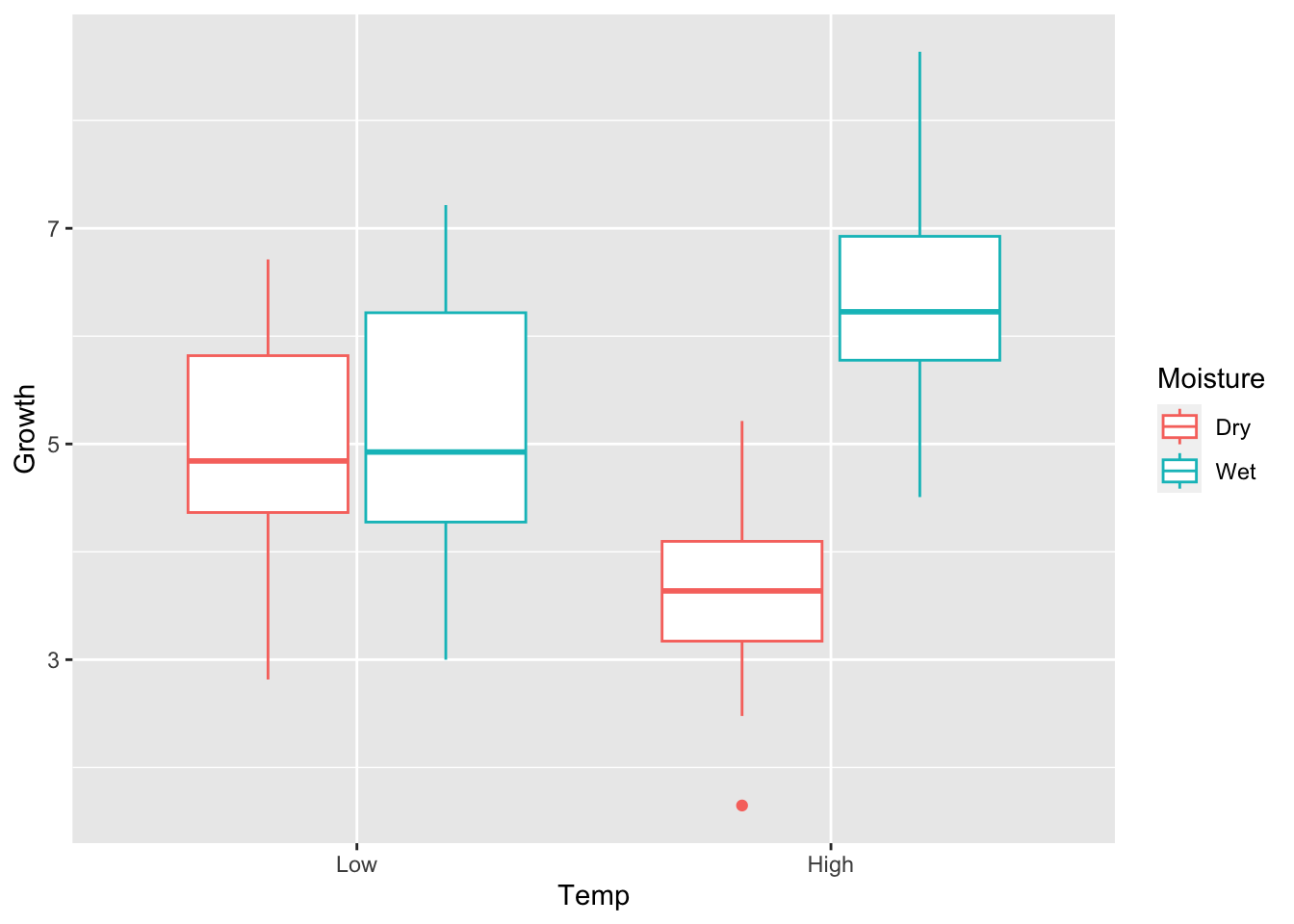
# INTERACTIONglobal=5beta_t=-1.25beta_m=0beta_intx=2.5sigma=1.0set.seed(5)y=NULLfor(iin1:length(Temp)){y[i]=global+beta_t*Temp[i]+beta_m*Moisture[i]+beta_intx*Temp[i]*Moisture[i]+rnorm(1, mean =0, sd =sigma)}# Store as data frametwo_way_df2=data.frame( Growth =y, Temp =factor(Temp, levels =c(0,1), labels =c("Low", "High")), Moisture =factor(Moisture, levels =c(0,1), labels =c("Dry", "Wet")))ggplot(two_way_df2)+geom_boxplot(aes(x =Temp, y =Growth, color =Moisture))
What wee see is that the effect of Temperature depends on the value of soil Moisture. In this case, as Temperature moves from Low to High, plant Growth declines if the soil is Dry, but Growth increases if the soil is Wet.
But those trends are just visual at this point. How do we quantify whether specific comparisons are statistically significant? We will again use the Tukey HSD! First, run the ANOVA and verify that there is a significant interaction.
aov_intx=aov(Growth~Temp+Moisture+Temp:Moisture, data =two_way_df2)summary(aov_intx)
The important part of the out put is $'Temp:Moisture', which shows the pairwise tests of the interactive effects. See if you can understand which differences are statistically significant, after accounting for multiple comparisons.
8.3 ANCOVA
ANCOVA is a variant of ANOVA, which stands for “Analysis of Covariance”. For one-way ANCOVA, we are analyzing the effect of one discrete (i.e., categorical) input variable, plus one continuous input variable. The “covariance” part refers to the fact that we’re trying to understand if the slope of the continuous input variable is the same or different between the levels of the discrete input variable.
For one-way ANCOVA, we have a single discrete input variable, and let’s assume the levels are 0 or 1. The model for one-way ANCOVA can then be written as: \[y_i = \mu_0 + \alpha_1 X_i + \beta_1 Z_i + \beta_2 X_i Z_i + \epsilon_i\] Here, \(\beta_1\) is the slope of \(Z\) when \(X=0\), but \(\beta_1 + \beta_2\) is the slope of \(Z\) when \(X=1\). If there is no interaction (i.e., \(\beta_2=0\)), then the slope of \(Z\) is the same for the two levels of \(X\).
Let’s continue with our example from two-way ANOVA, where we have Temperature and soil Moisture. However, for ANCOVA, we will assume that Temperature is a continuous input variable, rather than a discrete one.
8.3.1 Create data set and model function
We are going to explore all four possible outcomes of the simple one-way ANCOVA. We will therefore create a static data set, as well as a function to simulate the outcome variable \(Y\), depending on the model parameters.
library(ggplot2)set.seed(7)n_rep=35# Dry, Wet (0, 1)Moisture=rep(0:1, each =n_rep)# Continuous TemperatureTemp=c(runif(n_rep, min =5, max =25),runif(n_rep, min =5, max =25))# Function to simulate observed datacalc_y_func=function(mu_0=0,alpha_1=0,beta_1=0,beta_2=0,sigma=1.0){y=NULLfor(iin1:length(Temp)){y[i]=mu_0+alpha_1*Moisture[i]+beta_1*Temp[i]+beta_2*Temp[i]*Moisture[i]+rnorm(1, mean =0, sd =sigma)}return(y)}
8.3.2 Main effect of Temperature
First, we’ll see what the data look like when we only have an effect of the continuous input variable, in this case Temperature.
set.seed(2)# 1. Only slope effectmu_0=5alpha_1=0beta_1=0.75beta_2=0sigma=2.25y1=calc_y_func(mu_0,alpha_1,beta_1,beta_2,sigma)# Store as data frameancova_df1=data.frame( Growth =y1, Temp =Temp, Moisture =factor(Moisture, levels =c(0,1), labels =c("Dry", "Wet")))ggplot(ancova_df1)+geom_point(aes(x =Temp, y =Growth, shape =Moisture, color =Moisture))
We can see that while there is clearly a linear effect of Temperature on plant Growth, there is no obvious difference between Dry and Wet soil Moisture.
Now, let’s use model simplification to statistically validate our visual interpretation of the data.
m1=aov(Growth~Temp+Moisture+Temp*Moisture, data =ancova_df1)summary(m1)
# We can try dropping the interactionm2=update(m1, .~.-Temp:Moisture)anova(m1, m2)
Analysis of Variance Table

Model 1: Growth ~ Temp + Moisture + Temp * Moisture
Model 2: Growth ~ Temp + Moisture
  Res.Df    RSS Df Sum of Sq      F Pr(>F)
1     66 438.35
2     67 452.99 -1   -14.641 2.2044 0.1424
# Notice how this F and p-value is the same from# the summary() table of m1. m3=update(m2, .~.-Moisture)summary(m3)
            Df Sum Sq Mean Sq F value Pr(>F)
Temp         1   1423  1422.8   205.9 <2e-16 ***
Residuals   68    470     6.9
---
Signif. codes:  0 '***' 0.001 '**' 0.01 '*' 0.05 '.' 0.1 ' ' 1
# Check the slope and interceptm3$coefficients
(Intercept)        Temp
   4.487613    0.787559
The model simplification validates that there is only an effect of Temperature, and the estimated slope matches our simulated value pretty closely.
8.3.3 Main effect of Moisture
Now, let’s assume there is no effect of Temperature, but there is a difference in the levels of Moisture.
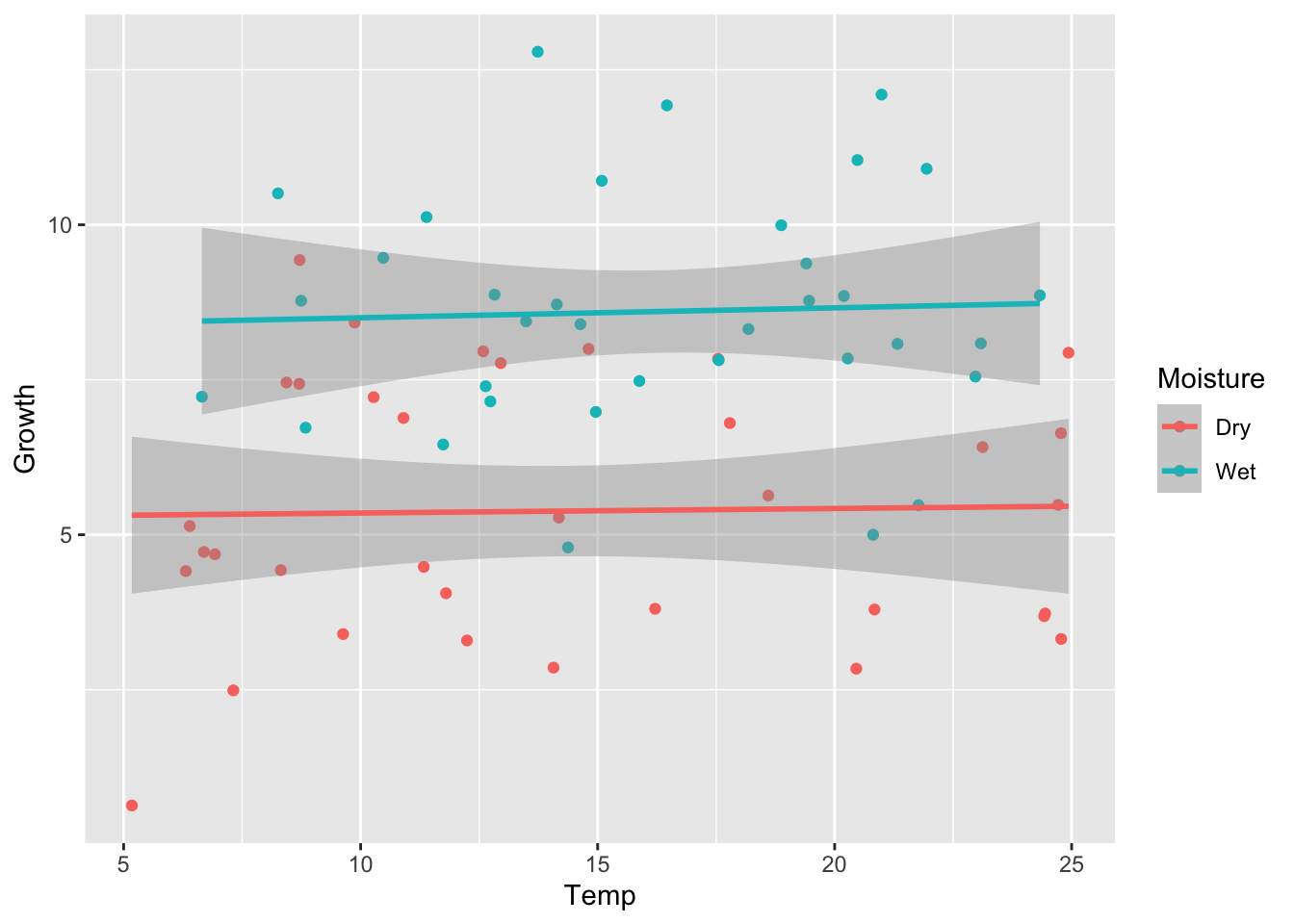
set.seed(5)# 2. Only factor effectmu_0=5alpha_1=4beta_1=0beta_2=0sigma=2.0y2=calc_y_func(mu_0,alpha_1,beta_1,beta_2,sigma)# Store as data frameancova_df2=ancova_df1ancova_df2$Growth=y2ggplot(ancova_df2)+geom_point(aes(x =Temp, y =Growth, shape =Moisture, color =Moisture))
We can see the difference in the means of Moisture levels, but no clear, linear Temperature effect. We will validate this with model simplification.
m1=aov(Growth~Temp+Moisture+Temp*Moisture, data =ancova_df2)summary(m1)
  Tukey multiple comparisons of means
    95% family-wise confidence level

Fit: aov(formula = Growth ~ Moisture, data = ancova_df2)

$Moisture
            diff      lwr      upr p adj
Wet-Dry 3.218663 2.264057 4.173269     0
The test shows that Wet soil leads to an approximately 3.2 value increase in plant Growth over dry soil, and this is a statistically significant difference (p-value is very low, near zero).
We can use ggplot2 to help us visualize this differnce more clearly.
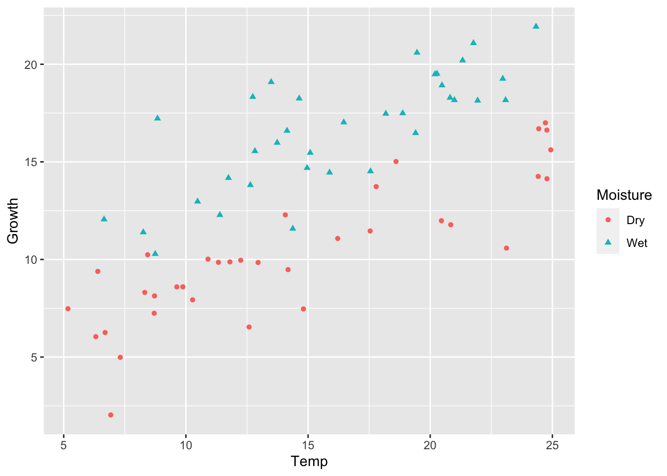
Now, let’s assume there is a linear effect of Temperature, and there is a difference in the levels of Moisture. But, there is still no interaction.
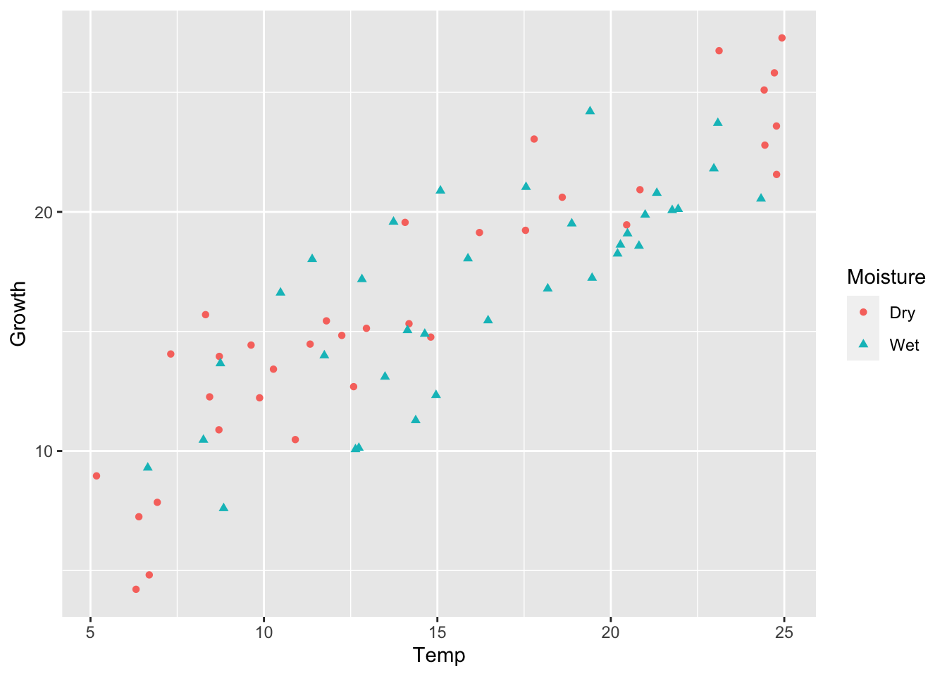
set.seed(1)# 3. Factor and Slope effectmu_0=3alpha_1=5beta_1=0.5beta_2=0sigma=2.0y3=calc_y_func(mu_0,alpha_1,beta_1,beta_2,sigma)# Store as data frameancova_df3=ancova_df1ancova_df3$Growth=y3ggplot(ancova_df3)+geom_point(aes(x =Temp, y =Growth, shape =Moisture, color =Moisture))
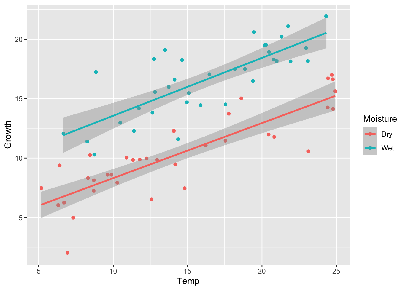
We can see the difference in the means of Moisture levels, and an obvious linear Temperature effect. Again, we will validate this with model simplification.
m1=aov(Growth~Temp+Moisture+Temp*Moisture, data =ancova_df3)summary(m1)
The test shows that Wet soil leads to an approximately 5.3 value increase in plant Growth over dry soil, and that Temperature has a similar positive, linear effect on plant Growth for both wet and dry soil.
We can use ggplot2 to help us visualize this difference more clearly.
8.3.5 Interaction between Temperature and Moisture
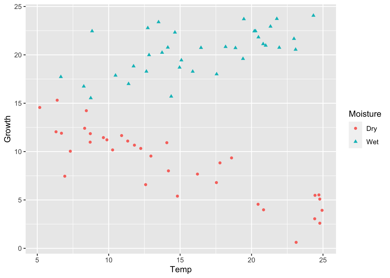
Finally, let’s assume there is an interaction between Moisture and Temperature.
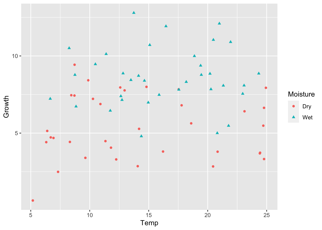
########################set.seed(1)# 4. Positive interactionmu_0=15alpha_1=0beta_1=-0.45beta_2=0.75sigma=2.0y4=calc_y_func(mu_0,alpha_1,beta_1,beta_2,sigma)# Store as data frameancova_df4=ancova_df1ancova_df4$Growth=y4ggplot(ancova_df4)+geom_point(aes(x =Temp, y =Growth, shape =Moisture, color =Moisture))
We can visually notice how the slope of Temperature depends on whether soil Moisture is Wet or Dry. But we need to conduct model simplification to validate this.
m1=aov(Growth~Temp+Moisture+Temp*Moisture, data =ancova_df4)summary(m1)
We see the model coefficients match well to our simulated values. Specifically, there is a positive interaction: the slope of Temperature when soil is Dry is negative (\(-0.49\)), but when the soil is Wet, the slope of temperature increases and becomes positive (\(-0.49 + 0.77 = 0.28\)).
# ANOVA {#sec-anova}## One-way ANOVARemember that Analysis of Variance (ANOVA) is using linear regression to analyze how discrete input variables affect an outcome. Because the input variables are comprised of discrete "levels" (e.g., treatment groups), we are really comparing how the mean of an outcome varies among discrete groups. This is therefore a generalization of two-sample $t$-tests to the case of more than two samples/groups. One-way ANOVA is the special case in which we only have one input variable, which has more than two "levels". The ANOVA linear model can be written in several ways, but for me the easiest way to think about is as follows:$$y_{i,l} = \mu_l + \epsilon_{i,l}$$$$\epsilon \sim N(0, \sigma^2 I)$$In this case $l = 1,\dots,L$, where $L$ is the number of levels in the input variable $x$, and $\mu_l$ is the mean outcome of group level, $l$. Thus, each data observation $y_{i,l}$ varies about a group level mean, with residuals $\epsilon_{i,l}$, which are normally and independently distributed. Perhaps this is easier to visualize and see the code. Let's simulate a case in which we have a single input variable $x$ that has 3 levels. ```{r}set.seed(5)n_levels =3n_obs_per_level =25# Construct Xx =rep(c(1:n_levels), each = n_obs_per_level)# Assign group-wise meansmus =NULLmus[1] =5.0mus[2] =7.5mus[3] =5.8sigma =2.5# residual sigma# Simulate data obsy =NULLfor(i in1:length(x)){ this_level = x[i] y[i] = mus[this_level] +# residual deviation from group-wise mean:rnorm(1, mean =0, sd = sigma)}# Store in data frameone_way_df =data.frame(y = y,x =factor(x) # store as factor/categorical)# Plot the means:## Defaults to boxplot() when x is discreteplot(y~x, data = one_way_df)```We can see that - at least visually - level 2 has a higher mean outcome than the other levels (e.g., $\bar{y}_2$ seems largest). Let's run the ANOVA model and see the summary. ```{r}# Use the aov() functionm_one_way =aov(y ~1+ x, data = one_way_df)summary(m_one_way)```### Manually calculate $F$As we can see, the `aov()` function is using an $F$-test to determine if any of the group-wise means differ from the global mean (see lecture materials on this topic). Indeed, based on the $p$-value, at least one group-wise mean is different. To verify our understand, as usual, let's manually calculate the $F$ test statistic and $p$-value.```{r}# First, we need to run the "null" model (intercept only)m_one_way_null =lm(y ~1, data = one_way_df)# Extract the residuals (errors)resid_full = m_one_way$residualsresid_null = m_one_way_null$residuals# Sum of Square Errors (SSE)sse_full =crossprod(resid_full)sse_null =crossprod(resid_null)# degrees of freedomn_obs =length(y)df_full = n_obs - n_levelsdf_null = n_obs -1# Calculate F_statf_test = ((sse_null - sse_full)/(df_null - df_full)) / (sse_full/df_full)# Degrees of freedom for the F distribution:df_numerator = df_null - df_fulldf_denominator = df_fullp_one_way =1-pf(f_test,df1 = df_numerator,df2 = df_denominator)# Compare to anova()f_test; p_one_waysummary_aov =summary(m_one_way)summary_aov[[1]]$`F value`; summary_aov[[1]]$`Pr(>F)````We see that our manual calculation of $F$ and the corresponding $p$-value match with the output of the `aov()` function, so we can verify we are understanding what `aov()` is doing.### Tukey HSDBut, which specific means differ from each other? To know this, we need to compute all pairwise differences between the group-wise means. Remember that for $L$ number of groups, we have $L(L-1)/2$ number of pairwise comparisons. We want to correct for multiple comparisons, so we don't inflate our risk of Type I errors. Therefore, we'll conduct a Tukey Honest Significant Difference (HSD) test. ```{r}TukeyHSD(m_one_way)```This test is looking at pairwise differences. For instance `2-1` is the difference between $x$ levels 2 and 1, and so on. The output reports the raw difference in means as `diff`, and then reports the lower and upper confidence limits of this difference as `lwr` and `upr`. These default to 95% confidence intervals, though the user can specify an option in the function to change this percentage confidence. Then the output reports the `p adj`, which is the adjusted $p$-value, adjusting for multiple comparisons. Here, we can conclude that while levels 1 and 3 are not different from one another, level 2 is different from both levels 1 and 3. This makes sense when we look at the boxplot (again).```{r}plot(y~x, data = one_way_df)```### Manually calculate $q$How does the Tukey HSD adjust for multiple comparisons? It uses a special hypothesis test, which has an associated probability distribution, `tukey`. Remember that we calculate a test statistic, $q$ for the difference between levels $i$ and $j$:$$q_{i,j} = \frac{|\bar{y}_i - \bar{y}_j|}{\sqrt{\hat{\sigma}^2_p/n}}$$Here, $\hat{\sigma}^2_p$ is the *pooled* variance of the whole outcome data set, $y$, and $n$ is the number of observations *per level*. This is why a **balanced design** is important; the test assumes that each level has the same number of observations. Let's manually calculate the $p$-value for the difference between group levels 2 and 1. ```{r}# Need to extract the data observations associated with all x levels, separatelythese_x_1 =which(x ==1)these_x_2 =which(x ==2)these_x_3 =which(x ==3)y_1 = y[these_x_1]y_2 = y[these_x_2]y_3 = y[these_x_3]# Calculate pooled variance for whole data set# Notice how this is not the same as var(y)pooled_var = (var(y_1)+var(y_2)+var(y_3))/3# Calculate q test statisticq_test =abs(mean(y_1) -mean(y_2)) /sqrt(pooled_var/n_obs_per_level)q_test# Degrees of freedom for q test statdf_q = n_obs - n_levels# Calculate p-valuep_2v1 =ptukey(q_test, nmeans =3,df = df_q, lower.tail =FALSE)p_2v1```We can see this $p$-value matches the first `p adj` from the `TukeyHSD()` output. ## Two-way ANOVATwo-way ANOVA is the special case in which we have exactly two input variables, each of which has two or more "levels". The two-way ANOVA linear model can be written in several ways. We'll start with the easiest case in which each of the two input variables only has two levels. This refers to a "2x2" experimental design. To be concrete, we'll use an example. We will simulate data for plant growth in which we manipulate Temperature (`Low` or `High`) and soil Moisture (`Dry` or `Wet`). We apply the 2x2 combination of these treatments which leads to four total treatments (e.g., Low-Dry, Low-Wet, etc.). We will apply each treatment combination to 25 plants and measure the outcome of Growth. In the following model structure, we will code Temperature as `Low == 0` and `High == 1`, and we will code soil Moisture as `Dry == 0` and `Wet == 1`. $$y_{i} = \mu + \beta_{\text{Temp}}\text{Temp} + \beta_{\text{Moist}}\text{Moist} + \beta_{\text{Intx}}\text{Temp}\text{Moist} + \epsilon_{i,l}$$$$\epsilon \sim N(0, \sigma^2 I)$$In the model structure, $\mu$ is a global mean for $y$ (i.e., across all treatments). Then, this global mean can be altered (i.e. affected by) the treatment combinations. $\beta_{\text{Temp}}$ and $\beta_{\text{Moist}}$ are the "main" effects and $\beta_{\text{Intx}}$ is the interactive effect. `Temp` and `Moist` are binary indicator variables (0/1), so, for instance, if Temperature is Low, `Temp == 0`, and so on. This means that $\beta_{\text{Temp}}$ only gets added to the global mean when `Temp == 1` (i.e., Temperature is High), and so on. The $\beta_{\text{Intx}}$ would get added to the global mean if both Temp and Moist are 1, so `High` Temperature and `Wet` Moisture. ### Only main effectsFirst, let's simulate a case in which we only have main effects, no interaction. Specifically, we will assume that the plant Growth declines under `High` Temperature, but that there is no effect of soil Moisture. Also, for data visualization, we will use the `ggplot2` package, because it is easier to customize. ```{r}library(ggplot2)# 2x2 design# Replicated 25 times# Low, High (0, 1)n_reps =25Temp =rep(0:1, each = n_reps*2)# Low, High (0, 1)Moisture =c(rep(0:1, each = n_reps),rep(0:1, each = n_reps))# Simulate different effects:set.seed(8)# Just main effectglobal =5beta_t =-1.25beta_m =0beta_intx =0sigma =1.0y =NULLfor(i in1:length(Temp)){ y[i] = global + beta_t * Temp[i] + beta_m * Moisture[i] + beta_intx * Temp[i] * Moisture[i] +rnorm(1, mean =0, sd = sigma)}# Store as data frametwo_way_df1 =data.frame(Growth = y,Temp =factor(Temp, levels =c(0,1), labels =c("Low", "High")),Moisture =factor(Moisture, levels =c(0,1), labels =c("Dry", "Wet")))ggplot(two_way_df1) +geom_boxplot(aes(x = Temp, y = Growth, color = Moisture))```Here, it is visually clear that higher temperatures lead to lower plant growth, but there is no clear effect of soil moisture, just as we simulated. Let's run the ANOVA model and see if the output makes sense.```{r}summary(aov(Growth ~ Temp + Moisture + Temp:Moisture,data = two_way_df1))```Indeed, we only see a main effect of `Temp`, and no main effect of `Moisture`, and no interactive effect (`Temp:Moisture`).### Interactive effectNow will simulate a case in which we have a main effect of temperature, similar to the above (Growth declines at `High` Temp). We will also add a positive interactive effect. This means that the effect of specific effects of temperature on growth will depend on the soil moisture content. Specifically, with a positive interactive effect, if Temperature is `High` and Moisture is `Wet`, then we will get an increase in Growth, rather than a decline. Let's see what this looks like visually. ```{r}# INTERACTIONglobal =5beta_t =-1.25beta_m =0beta_intx =2.5sigma =1.0set.seed(5)y =NULLfor(i in1:length(Temp)){ y[i] = global + beta_t * Temp[i] + beta_m * Moisture[i] + beta_intx * Temp[i] * Moisture[i] +rnorm(1, mean =0, sd = sigma)}# Store as data frametwo_way_df2 =data.frame(Growth = y,Temp =factor(Temp, levels =c(0,1), labels =c("Low", "High")),Moisture =factor(Moisture, levels =c(0,1), labels =c("Dry", "Wet")))ggplot(two_way_df2) +geom_boxplot(aes(x = Temp, y = Growth, color = Moisture))```What wee see is that the effect of Temperature depends on the value of soil Moisture. In this case, as Temperature moves from `Low` to `High`, plant Growth declines if the soil is `Dry`, but Growth increases if the soil is `Wet`. But those trends are just visual at this point. How do we quantify whether specific comparisons are statistically significant? We will again use the Tukey HSD! First, run the ANOVA and verify that there is a significant interaction.```{r}aov_intx =aov(Growth ~ Temp + Moisture + Temp:Moisture,data = two_way_df2)summary(aov_intx)```Indeed, the interaction is significant, so now we need to figure out which specific differences among covariate levels exist. ```{r}TukeyHSD(aov_intx)```The important part of the out put is `$'Temp:Moisture'`, which shows the pairwise tests of the interactive effects. See if you can understand which differences are statistically significant, after accounting for multiple comparisons. ## ANCOVAANCOVA is a variant of ANOVA, which stands for "Analysis of **Co**variance". For one-way ANCOVA, we are analyzing the effect of one discrete (i.e., categorical) input variable, plus one continuous input variable. The "covariance" part refers to the fact that we're trying to understand if the slope of the continuous input variable is the same or different between the levels of the discrete input variable.For one-way ANCOVA, we have a single discrete input variable, and let's assume the levels are 0 or 1. The model for one-way ANCOVA can then be written as:$$y_i = \mu_0 + \alpha_1 X_i + \beta_1 Z_i + \beta_2 X_i Z_i + \epsilon_i$$Here, $\beta_1$ is the slope of $Z$ when $X=0$, but $\beta_1 + \beta_2$ is the slope of $Z$ when $X=1$. If there is no interaction (i.e., $\beta_2=0$), then the slope of $Z$ is the same for the two levels of $X$. Let's continue with our example from two-way ANOVA, where we have Temperature and soil Moisture. However, for ANCOVA, we will assume that Temperature is a *continuous* input variable, rather than a discrete one. ### Create data set and model functionWe are going to explore all four possible outcomes of the simple one-way ANCOVA. We will therefore create a static data set, as well as a function to simulate the outcome variable $Y$, depending on the model parameters.```{r}library(ggplot2)set.seed(7)n_rep =35# Dry, Wet (0, 1)Moisture =rep(0:1, each = n_rep)# Continuous TemperatureTemp =c(runif(n_rep, min =5, max =25),runif(n_rep, min =5, max =25))# Function to simulate observed datacalc_y_func =function(mu_0 =0,alpha_1 =0,beta_1 =0,beta_2 =0,sigma =1.0){ y =NULLfor(i in1:length(Temp)){ y[i] = mu_0 + alpha_1 * Moisture[i] + beta_1 * Temp[i] + beta_2 * Temp[i] * Moisture[i] +rnorm(1, mean =0, sd = sigma) }return(y)}```### Main effect of TemperatureFirst, we'll see what the data look like when we only have an effect of the continuous input variable, in this case Temperature. ```{r}set.seed(2)# 1. Only slope effectmu_0 =5alpha_1 =0beta_1 =0.75beta_2 =0sigma =2.25y1 =calc_y_func( mu_0,alpha_1,beta_1, beta_2,sigma)# Store as data frameancova_df1 =data.frame(Growth = y1,Temp = Temp,Moisture =factor(Moisture, levels =c(0,1), labels =c("Dry", "Wet")))ggplot(ancova_df1) +geom_point(aes(x = Temp, y = Growth, shape = Moisture, color = Moisture))```We can see that while there is clearly a linear effect of Temperature on plant Growth, there is no obvious difference between Dry and Wet soil Moisture. Now, let's use model simplification to statistically validate our visual interpretation of the data. ```{r}m1 =aov(Growth ~ Temp + Moisture + Temp*Moisture, data = ancova_df1)summary(m1)# We can try dropping the interactionm2 =update(m1, .~. -Temp:Moisture)anova(m1, m2)# Notice how this F and p-value is the same from# the summary() table of m1. m3 =update(m2, .~. -Moisture)summary(m3)# Check the slope and interceptm3$coefficients```The model simplification validates that there is only an effect of Temperature, and the estimated slope matches our simulated value pretty closely. ### Main effect of MoistureNow, let's assume there is no effect of Temperature, but there is a difference in the levels of Moisture. ```{r}set.seed(5)# 2. Only factor effectmu_0 =5alpha_1 =4beta_1 =0beta_2 =0sigma =2.0y2 =calc_y_func( mu_0,alpha_1,beta_1, beta_2,sigma)# Store as data frameancova_df2 = ancova_df1ancova_df2$Growth = y2ggplot(ancova_df2) +geom_point(aes(x = Temp, y = Growth, shape = Moisture, color = Moisture))```We can see the difference in the means of Moisture levels, but no clear, linear Temperature effect. We will validate this with model simplification. ```{r}m1 =aov(Growth ~ Temp + Moisture + Temp*Moisture, data = ancova_df2)summary(m1)m2 =update(m1, .~. - Temp:Moisture)summary(m2)m3 =update(m2, .~. - Temp)summary(m3)```Indeed, the model with only Moisture is best. We can then use Tukey HSD to validate the specific differences in the Moisture levels. ```{r}TukeyHSD(m3)```The test shows that Wet soil leads to an approximately 3.2 value increase in plant Growth over dry soil, and this is a statistically significant difference (p-value is very low, near zero).We can use `ggplot2` to help us visualize this differnce more clearly. ```{r}ggplot(ancova_df2, aes(x = Temp, y = Growth, color = Moisture)) +geom_point() +geom_smooth(method ="lm")```### Main effects of Temperature and MoistureNow, let's assume there is a linear effect of Temperature, and there is a difference in the levels of Moisture. But, there is still no interaction.```{r}set.seed(1)# 3. Factor and Slope effectmu_0 =3alpha_1 =5beta_1 =0.5beta_2 =0sigma =2.0y3 =calc_y_func( mu_0,alpha_1,beta_1, beta_2,sigma)# Store as data frameancova_df3 = ancova_df1ancova_df3$Growth = y3ggplot(ancova_df3) +geom_point(aes(x = Temp, y = Growth, shape = Moisture, color = Moisture))```We can see the difference in the means of Moisture levels, and an obvious linear Temperature effect. Again, we will validate this with model simplification. ```{r}m1 =aov(Growth ~ Temp + Moisture + Temp*Moisture, data = ancova_df3)summary(m1)m2 =update(m1, .~. - Temp:Moisture)summary(m2)# m2 is bestm2$coefficients```The test shows that Wet soil leads to an approximately 5.3 value increase in plant Growth over dry soil, and that Temperature has a similar positive, linear effect on plant Growth for both wet and dry soil. We can use `ggplot2` to help us visualize this difference more clearly. ```{r}ggplot(ancova_df3, aes(x = Temp, y = Growth, color = Moisture)) +geom_point() +geom_smooth(method ="lm")```### Interaction between Temperature and MoistureFinally, let's assume there is an interaction between Moisture and Temperature. ```{r}########################set.seed(1)# 4. Positive interactionmu_0 =15alpha_1 =0beta_1 =-0.45beta_2 =0.75sigma =2.0y4 =calc_y_func( mu_0,alpha_1,beta_1, beta_2,sigma)# Store as data frameancova_df4 = ancova_df1ancova_df4$Growth = y4ggplot(ancova_df4) +geom_point(aes(x = Temp, y = Growth, shape = Moisture, color = Moisture))```We can visually notice how the slope of Temperature depends on whether soil Moisture is Wet or Dry. But we need to conduct model simplification to validate this. ```{r}m1 =aov(Growth ~ Temp + Moisture + Temp*Moisture, data = ancova_df4)summary(m1)# cannot drop interaction# full model is bestm1$coefficients```We see the model coefficients match well to our simulated values. Specifically, there is a positive interaction: the slope of Temperature when soil is Dry is negative ($-0.49$), but when the soil is Wet, the slope of temperature increases and becomes positive ($-0.49 + 0.77 = 0.28$). Let's visualize this more clearly with `ggplot2`.```{r}ggplot(ancova_df4, aes(x = Temp, y = Growth, color = Moisture)) +geom_point() +geom_smooth(method ="lm")```